PERT distribution leads to overconfidence in outcomes

In my last post, I explored the phenomenon that while most activities on projects are delivered on time, most projects are delivered late. I introduced the concept of long-tails in distributions and how it’s the activities that reside in these long-tails that cause most of the delay in projects.

Given this, it’s critical that we learn how to model these events when undertaking schedule risk forecasting, yet the status quo in QSRA disregards these types of events leading to project managers being unprepared for events that could derail their projects.

In this post, I want to explore the way uncertainty modeling is done in QSRA, in particular looking at the impact that using one of the 3 bounded distributions described in my previous post has on the overall project forecast. As a reminder, the 3 distributions you typically see used are the following:

Note that they are bounded because of the limits that are imposed by a human when defining these distributions.

PERT vs Lognormal Distribution

What happens if instead of using a bounded distribution to model activity durations, we use an unbounded distribution? What impacts does that have on our overall project forecasts when we undertake QSRA?

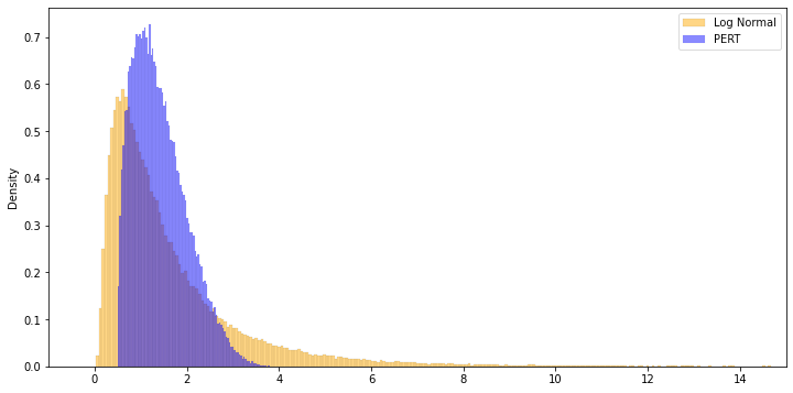
A good candidate for an unbounded distribution to model activity durations is the Lognormal distribution, pictured below.

Some nice properties that make the Lognormal distribution suitable is that it is strictly positive (so no need to worry about negative durations) and it allows for non-zero probability of large delays. That means that we can begin to assign a very small probability to large delays instead of completely disregarding them.

When compared to the PERT distribution we notice that there is a large overlap around the area of “on-time” completion, as we would expect. The main difference is of course the areas outside of the bounds set in the PERT distribution.

Armed with these two distributions, we can begin to compare how uncertainty is propagated through the project as we sample 1000s of times for activities taking into account their dependencies.

Viewing a project as a graph

At its simplest, a project is a set of tasks that are joined by links (specifying dependencies between two tasks). This can be easily visualized as a network like in the image below. Each point (or node) is a task, with an associated duration, and the edges that connect them are the dependencies.

Broken down even further, project graphs are made up of two patterns:

Linear Chain: Task A can only start once all the previous tasks are completed i.e. after the sum of all preceding durations

Merge Points: Task B can only start once the last of all preceding tasks finishes i.e. after the max of all preceding durations

Therefore, if we want to understand how uncertainty is propagated for an entire project, we can begin by investigating these smaller cases and use the findings to investigate the overall project forecast. The subsequent graphs below show the resulting distribution for Task A and Task B in the examples above as we increase the number of predecessors, for both the PERT distribution and Lognormal distribution.

There is nothing very surprising or different in the linear chain case. As we add more activities to the chain, the distribution shifts to the right since we’re adding more duration. On top of that, the distribution becomes wider because each preceding activity adds some uncertainty to the overall sum. Note that in the case of the lognormal distribution, the distribution becomes wider at a faster rate because of the probability of events that lay outside of the bounds of the PERT distribution.

On the other hand, the merge points case is much more interesting and surprising. As we increase the number of predecessors for Task B, the resulting distribution in the Lognormal case shifts to the right and gets wider. This is because, as we add more predecessors, we’re increasing the chance that at least one of them is an extreme event, therefore making the distribution wider. However, the resulting distribution in the PERT case actually becomes narrower! This means that the start of Task A becomes more certain the more predecessors Task A has! Why does this happen? Similar to the Lognormal case, the more predecessors we add, the higher chance there is of an extreme event occurring. Except, in this case, there is an upper bound to the original distribution, meaning that we are increasing the chances that at least one of the tasks will equal that upper bound, resulting in a more “confident” forecast.

The ramifications of this simple phenomenon could be quite wicked because every merge point in a project schedule will actually decrease the uncertainty in our resulting forecast leading to a false confidence in the overall project forecast. When this comparison is carried out for a full project forecast, in a project with 1000s of activities, you get the distributions below. Not only are the distributions quite far apart, but also the overall uncertainty with regards to the project outcome changes significantly when using a bounded vs an unbounded distribution.

Conclusions

I started this article series by highlighting the seeming paradox that while most activities are delivered on time, most projects are delayed. We see that extreme events don’t just exist, they are prevalent across the construction industry, yet they are not given enough consideration when it comes to forecasting our project end dates. In fact, we are not just ignoring them, we are creating a false confidence in our forecasts by using bounded distributions! This false confidence can lead to misallocation of resources, reputational damage and financial repercussions to name a few.

Is using a distribution such as the Lognormal distribution the right solution? Probably not. While it may give a better picture of risk in a project, it might not be fit for modeling all kinds of activities in the world. That’s why at nPlan we’ve taken the approach of using machine learning to learn unique activity distributions for each activity based on millions of historical data points.